Key takeaways
- Efficiency in transformer equipment typically ranges from 97.0% for small distribution units to over 99.7% for large utility power transformers.
- Maximum efficiency occurs at the specific operating load factor where variable winding load losses equal constant core losses.
- The standard efficiency of a transformer formula evaluates active output power against total losses: Efficiency = Output Power / (Output Power + Core Loss + Load Loss).
- Distribution transformers are typically engineered for peak efficiency at 40% to 50% load to maximise all-day operational energy savings under cyclic loading.
- Harmonics and elevated operating temperatures reduce actual system efficiency by generating supplementary eddy-current losses and raising conductor DC resistance.
Quick answer: Operational efficiency in transformer equipment measures the ratio of useful active output power delivered to the load against the total active electrical power absorbed from the source. Modern power and distribution units operate with exceptionally high efficiencies, typically spanning between 97.5% and 99.7% depending on asset rating, core metallurgy, and loading profile.
Because electrical transformers contain no moving mechanical parts, their losses are purely electromagnetic and thermal. Even a minor variation of 0.2% in transformer efficiency yields significant financial and environmental consequences over an operating lifecycle spanning 30 to 40 years. Industrial facility managers, substation designers, and utility planners calculate these figures rigorously during procurement through loss capitalisation formulas. Determining real-world asset performance requires an in-depth understanding of standard testing methods, loss allocation, and international compliance benchmarks such as IEC 60076-1 and IEEE C57.12.00.
Understanding efficiency in transformer engineering
Efficiency in transformer systems represents the proportion of input power successfully transmitted to the secondary circuit without dissipating as heat within the core or windings. Unlike rotating machinery, where friction and windage induce substantial mechanical drag, transformers convert alternating current through electromagnetic induction governed by Faraday's law. Consequently, energy dissipation is strictly limited to magnetic core degradation and resistive conductor excitation.
Transformer losses are divided into two distinct engineering classifications:
- No-load losses (Core losses): These constant losses occur continuously whenever the primary winding is energised, regardless of whether the secondary circuit is supplying power to an external load. No-load dissipation comprises hysteresis loss (caused by the cyclic reversal of magnetic domains in electrical steel laminations) and eddy-current loss (circulating currents induced inside the core material). Engineers minimise these using high-grade, cold-rolled grain-oriented (CRGO) silicon steel or amorphous metal alloys.
- Load losses (Copper losses): These variable losses depend directly on the square of the operational load current ($I^2R$). They encompass direct resistive dissipation within primary and secondary windings, eddy-current heating within the conductors, and stray flux coupling into mechanical clamping structures and the transformer tank walls.
When engineering an installation, sizing the equipment correctly using a comprehensive transformer sizing calculator guide ensures the unit operates consistently within its optimum efficiency envelope rather than running under-loaded or thermally saturated.
What are common efficiencies for transformers?
Common efficiencies for transformers typically span 97.0% to 99.0% for medium-voltage distribution units (50 kVA to 2,500 kVA) and exceed 99.5% to 99.75% for transmission-class power transformers rated above 20 MVA. Dry-type cast-resin units generally deliver slightly lower baseline efficiencies than equivalent mineral-oil-immersed units due to differences in core footprint, air clearances, and dielectric thermal dissipation properties.
Regulatory frameworks such as the European Union Ecodesign Directive (EN 50588-1 Tier 2) and the United States Department of Energy (DOE 10 CFR Part 431) establish mandatory minimum operational efficiency metrics. The following benchmark values reflect typical high-efficiency three-phase liquid-immersed transformers operating at standard reference temperatures (75°C) and rated voltage:
| Nominal Rating (kVA) | Typical Core Loss (W) | Full Load Loss @ 75°C (W) | Efficiency @ 50% Load (0.8 PF) | Efficiency @ 100% Load (1.0 PF) | Efficiency @ 100% Load (0.8 PF) |
|---|---|---|---|---|---|
| 100 kVA | 145 | 1,250 | 98.86% | 98.62% | 98.28% |
| 250 kVA | 300 | 2,350 | 99.12% | 98.95% | 98.69% |
| 500 kVA | 510 | 3,900 | 99.26% | 99.13% | 98.91% |
| 1,000 kVA | 850 | 7,600 | 99.32% | 99.16% | 98.95% |
| 1,600 kVA | 1,200 | 11,500 | 99.37% | 99.21% | 99.02% |
| 2,500 kVA | 1,700 | 16,500 | 99.41% | 99.28% | 99.10% |
| 10,000 kVA | 5,800 | 48,000 | 99.64% | 99.47% | 99.33% |
| 31,500 kVA | 14,500 | 115,000 | 99.73% | 99.59% | 99.49% |
To evaluate how these values translate across specific operating voltages, see our detailed technical breakdown on how transformers are rated in industrial power distribution networks.
Efficiency of a transformer formula and calculation methodology
The efficiency of a transformer formula defines operational performance as the ratio of true output power ($P_{out}$) to total active input power ($P_{in}$), expressed as a percentage: $\eta = (P_{out} / P_{in}) \times 100\%$. Because input power equals the sum of secondary output power and internal losses, the formula is universally stated in electrical engineering as:
$$\eta = \frac{P_{out}}{P_{out} + P_0 + P_k(x)^2} \times 100\%$$
Where the mathematical variables represent:
- $P_{out}$: Active output power delivered to the load, calculated as $S \times x \times \cos\phi$ (in kW).
- $S$: Nameplate apparent power rating of the transformer (in kVA).
- $x$: Per-unit load factor, representing actual load divided by rated load (e.g., $x = 0.5$ for 50% loading).
- $\cos\phi$: Power factor of the connected electrical load.
- $P_0$: No-load core loss (in kW), independent of load.
- $P_k$: Full-load copper loss at rated reference temperature (in kW).
Worked Engineering Example: Consider a 1,000 kVA substation transformer with a tested no-load loss ($P_0$) of 0.85 kW and full-load loss ($P_k$) of 7.6 kW. Calculate its efficiency when delivering power at 60% loading ($x = 0.6$) with an inductive power factor of 0.85:
- Calculate secondary active power: $P_{out} = 1,000\text{ kVA} \times 0.6 \times 0.85 = 510\text{ kW}$.
- Calculate variable load losses at 60% loading: $P_{loss,load} = 7.6\text{ kW} \times (0.6)^2 = 7.6 \times 0.36 = 2.736\text{ kW}$.
- Sum the total losses: $P_{total} = P_0 + P_{loss,load} = 0.85\text{ kW} + 2.736\text{ kW} = 3.586\text{ kW}$.
- Calculate efficiency: $\eta = (510 / (510 + 3.586)) \times 100\% = (510 / 513.586) \times 100\% = 99.302\%$.
Mathematically, maximum efficiency occurs when the variable load losses equal the constant no-load losses: $x^2 \times P_k = P_0$. Rearranging this equation reveals the exact loading ratio where maximum efficiency is achieved: $x_{max} = \sqrt{P_0 / P_k}$. For this example, $x_{max} = \sqrt{0.85 / 7.6} = \sqrt{0.1118} = 0.334$ (or 33.4% loading).
Step-by-step procedure to determine transformer efficiency from factory test reports
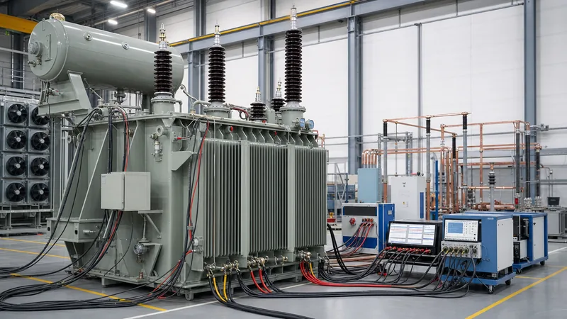
Determining true operational transformer efficiency requires extracting empirical test values from certified Factory Acceptance Test (FAT) reports and recalculating them to match real site conditions. Performing the physical validation steps is covered in our guide on how to test a transformer.
To calculate site-specific efficiency directly from test certificates, execute the following technical procedure:
- Extract the open-circuit test values: Obtain the no-load loss figure ($P_0$, in watts) measured during the open-circuit test conducted at 100% rated secondary voltage and nominal system frequency.
- Extract the short-circuit test values: Obtain the load loss figure ($P_k$, in watts) measured during the short-circuit test at rated primary current, noting the reference winding temperature (standardised at 75°C for liquid-immersed or 120°C/145°C for dry-type insulation classes).
- Correct for site operating temperature: If the unit operates continuously at an average winding temperature ($\theta_2$) different from the reference test temperature ($\theta_1$), correct the load loss using resistance adjustment formulas: $R_2 = R_1 \times (234.5 + \theta_2) / (234.5 + \theta_1)$ for electrolytic copper conductors.
- Determine your operational load factor ($x$): Calculate the ratio of your site demand apparent power to the transformer nameplate kVA rating ($x = S_{site} / S_{rated}$).
- Scale the thermal load losses: Multiply the temperature-corrected rated load loss by the square of the calculated load factor ($P_{load} = x^2 \times P_k$).
- Establish the operating power factor: Measure or assign the active displacement power factor ($\cos\phi$) of your plant facility.
- Compute the instantaneous operating efficiency: Substitute the adjusted parameters into the primary efficiency equation to establish operational performance under prevailing substation conditions.
Factors affecting transformer efficiency in real-world networks
Real-world transformer efficiency is governed primarily by operating load profile, service temperature, load power factor, and non-linear harmonic distortion. Factory test certificates record loss values under pure sinusoidal voltage and balanced linear resistive-inductive loads, which rarely mirror real industrial environments.
Key site variables impacting efficiency include:
- Operating Load Factor: Because copper losses scale with the square of the current, operating a transformer continuously above 80% to 90% load causes variable losses to surge, depressing operational efficiency. Conversely, running heavily under-loaded units (below 20%) reduces efficiency because fixed no-load core losses dominate the power balance.
- System Power Factor ($\\cos\phi$): As load power factor drops from unity (1.0) to inductive levels such as 0.70 or 0.80, the transformer must deliver higher current to support identical active power (kW). The resulting surge in $I^2R$ resistive heating lowers efficiency significantly.
- Harmonic Currents and Non-Linear Loads: Variable frequency drives (VFDs), server data centres, and uninterruptible power systems draw non-sinusoidal currents rich in 5th, 7th, and 11th harmonics. Harmonic frequencies amplify winding eddy-current losses in proportion to the square of the harmonic frequency ($f^2$), necessitating K-factor derating to prevent overheating and premature thermal aging.
- Internal Impedance and Regulation: As documented in our technical guide on transformer impedance calculations, an engineer must balance short-circuit current limitation against operating load losses when specifying short-circuit impedance percentage (%Z).
All-day efficiency vs nameplate efficiency for distribution networks
All-day efficiency is the ratio of total active energy output in kilowatt-hours (kWh) over a continuous 24-hour duty cycle to the total electrical energy input in kWh over the same period. In contrast to instantaneous nameplate efficiency, which assumes steady-state constant loading, all-day efficiency reflects real-world commercial, residential, and rural distribution performance.
Distribution transformers remain continuously connected to the utility network 24 hours a day, drawing constant no-load core excitation losses. However, actual customer demand fluctuates dramatically, often peaking for only 3 to 5 hours daily and idling at 15% to 25% load overnight. Under these variable dynamics, a unit with low full-load copper losses but high no-load core losses will exhibit poor 24-hour energy performance.
The engineering formula for all-day efficiency is expressed as:
$$\eta_{all-day} = \frac{\sum (P_{out, t} \times t)}{\sum (P_{out, t} \times t) + (P_0 \times 24) + \sum (x_t^2 \times P_k \times t)} \times 100\%$$
For this reason, utility-grade distribution transformers are engineered intentionally with a high ratio of load loss to no-load loss ($P_k / P_0 \approx 5:1 \text{ to } 8:1$). This design pushes the maximum efficiency inflection point down to 35%–50% average loading, minimising cumulative 24-hour kilowatt-hour losses.
Next steps: specifying and sourcing
When specifying high-efficiency power equipment, always supply manufacturers with your exact site load profile, operational power factor, and required loss capitalisation figures (A and B factors) alongside primary/secondary voltages and vector groups. Modern projects requiring high operational uptime benefit from precision-engineered power transformers and rugged, hermetically sealed oil-immersed transformers built to strict IEC, IEEE, and Ecodesign thresholds.
Our global engineering department designs and validates liquid-immersed, dry-type, and prefabricated substation systems tailored to low lifecycle operating costs. Submit your single-line diagrams (SLDs) and technical schedules directly through our transformer quotation portal to receive factory test loss data, compliance calculations, and competitive project pricing.
Frequently asked questions
what are common efficiencies for transformers
Common efficiencies for transformers range between 97.0% and 99.0% for medium-voltage distribution units and exceed 99.5% to 99.75% for large transmission power transformers. High-power units achieve near-unity performance because their large electromagnetic cross-sections dramatically reduce relative core and winding resistance.
What is the formula for calculating transformer efficiency?
The efficiency of a transformer formula is defined as Output Power divided by Input Power, represented as: Efficiency = (Pout / (Pout + P0 + Pk * x^2)) * 100%. Pout is the active load in kW, P0 is the constant core loss, Pk is the full-load copper loss, and x is the operating load factor.
At what load is transformer efficiency at its maximum?
Transformer efficiency reaches its maximum point when variable copper losses equal constant core losses (Pk * x^2 = P0). In distribution units, engineers deliberately design this crossover to occur between 35% and 50% of rated capacity to optimise energy performance under fluctuating daily load cycles.
Why is a transformer not 100% efficient?
A transformer cannot achieve 100% efficiency due to inherent thermodynamic and electromagnetic losses within its active parts. These consist of core hysteresis losses, circulating eddy-current heating within steel laminations and copper conductors, dielectric heating in insulation, and stray magnetic flux leaking into mechanical support structures.
How does power factor affect transformer efficiency?
A lower load power factor directly decreases operational transformer efficiency. When supplying a low power factor load, the transformer must deliver higher current to supply the same real power (kW), significantly increasing I^2R winding resistive heating losses while active output power remains unchanged.
What is the difference between ordinary efficiency and all-day efficiency?
Ordinary efficiency measures instantaneous active power performance under a specific steady-state load, whereas all-day efficiency calculates the ratio of total electrical energy output to energy input in kilowatt-hours (kWh) over a full 24-hour operating period under variable load conditions.
Tags: efficiency in transformer what are common efficiencies for transformers efficiency of a transformer formula transformer losses transformer testing